K-D tree fundamentals

TODO: what is a K-D tree

The nanoflann library is used within teqpflsh due to its computational efficiency.

The L2TreeHolder class makes a copy of the data for the tree to ensure that the lifetime of the data copied into the holder is longer than the tree itself. The underlying L2Tree object obtained via the .tree attribute then makes a reference to the data held in the holder class.

import numpy as np
import teqpflsh
import matplotlib.pyplot as plt

def boxpoly(*, top, bottom, left, right, ptr):
    X = np.array([left, right, right, left, left])
    Y = np.array([bottom, bottom, top, top, bottom])
    return ptr.makeclosedpolygon(X, Y)

ptr = teqpflsh.GeometryFactoryHolder()

# Polygon for the shifted circle
t = np.linspace(0, 2*np.pi, 10000)
X = 0.5 + 0.3*np.cos(t)
Y = 0.3*np.sin(t)
poly1 = ptr.makeclosedpolygon(X, Y)
poly2 = boxpoly(left=0, right=1, bottom=0, top=1, ptr=ptr)

# Polygon for the square [0,1]x[0,1] minus small circle
poly = poly2.difference(poly1)
X, Y = poly.getXY()

def do_one(*, NKD, Nsample, plot=False, close=True):
    def get_random(NKD):
        """ Random points for the tree """
        XX, YY = [], []
        while len(XX) < NKD:
            x_, y_ = np.random.random(2)
            pt = ptr.createPoint(float(x_), float(y_))
            if poly.containsPoint(pt):
                XX.append(x_)
                YY.append(y_)
        return XX, YY
    XX, YY = get_random(NKD)

    if plot:
        plt.plot(X, Y, 'k')
        plt.plot(XX, YY, '.', ms=5)

    holder = teqpflsh.L2TreeHolder(np.array(XX), np.array(YY), 10)
    tree = holder.tree

    xsample, ysample = get_random(Nsample)
    d2 = [tree.get_nearest_indexd2(x_, y_)[1] for x_, y_ in zip(xsample, ysample)]

    if plot:
        plt.axis('off')
        plt.axis('equal');
        if close:
            plt.close()

    return np.mean(np.array(d2)**0.5), tree.get_used_bytes()

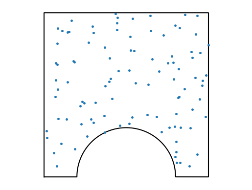
Here is a small number of “lighthouse” points randomly distributed in the domain. A random point is first pulled from [0,1]x[0,1] and checked whether it is within the domain or not. This so-called point-in-polygon problem is quite slow (relatively).

do_one(NKD=100, Nsample=100, plot=True, close=False);

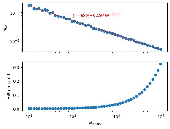
As you increase the number of points \(N\) inside the domain, the distance to the nearest point goes down like \(N^{-1/2}\) and in general the scaling should be like \(N^{-1/D}\) where \(D\) is the number of spatial dimensions (I think).

The required memory is linear with the number of points in the K-D tree(!)

Ntrees = np.geomspace(10, 10**4, dtype=int)

fig, (ax1, ax2) = plt.subplots(2, 1, sharex=True)

d2s = [do_one(NKD=NKD_, Nsample=10**3)[0] for NKD_ in Ntrees]
ax1.plot(Ntrees, d2s, 'o')

pf = np.polyfit(np.log(Ntrees), np.log(d2s), 1)
xx = np.geomspace(np.min(Ntrees), np.max(Ntrees), 1000)
ax1.plot(xx, np.exp(np.polyval(pf, np.log(xx))), dashes=[2,2], color='r')
ax1.text(100, 0.07, rf'$y=\exp({pf[1]:0.3f})N^{{{pf[0]:0.3f}}}$', color='r')

ax1.set_xscale('log')
ax1.set_yscale('log')
ax1.set(ylabel=r'$d_{NN}$')

MiBs = [do_one(NKD=NKD_, Nsample=10**3)[1]/1024**2 for NKD_ in Ntrees]
ax2.plot(Ntrees, MiBs, 'o')
ax2.set(xlabel=r'$N_{\rm points}$', ylabel='MiB required');

# del ptr